How a seemingly simple soldering issue led to a host of process questions.

Just the other day I was walking through the maze of cubes that I call home when an interesting comment caught my ear. The conversation was on how to solder a wire to a flexible printed circuit. How could it be possible that in this day and age when FPC assembly is common, and at times quite advanced, there would be a need to discuss how to solder a wire to an FPC? As I listened, it became clear this was not an ordinary solder-the-wire-to-a-board application. This was a micro-coax cable terminated to the FPC through solder joints to the copper circuitry directly, rather than through a board-mounted connector.

Let me frame the application: We wanted to take advantage of a very thin multilayer circuit populated with active and passive components in order to fit the interconnect into an extremely thin device – a perfect application for an FPCA. The trouble was, the micro-coax (coaxial) cable was the thickest component in the assembly, and the associated solder joint height was driving the overall Z height of the FPCA beyond the devices’ height requirement. How did we solve this? Let me walk you through some of the techniques we tried in order to reduce FPCA thickness, and share the solution we ultimately used.

Here’s our parameters:

• Both the inner cable and outer conductor required a solder connection.
• The solder height requirement was 80µm max.
• The gap between inner cable and solder pad needed to be reduced as much as possible.
• We needed to produce 150,000 per week.

Here are the choices we considered:

Good old-fashioned hand soldering. Hand soldering was used for the first design verification run. We knew it lacks the capability or volume scale needed for the final production unit, but it did allow us to get parts to the customer to start design evaluation, while we continued our evaluation of available processing options that exhibit solder volume.

Surface mount technology. SMT process for solder paste and reflow is the industry standard, exhibiting controlled paste volume, accurate paste placement, and appropriate throughput/cost for mass production. I had thought this would be the ideal solution, as the FPCA had many other components to be mounted on the side where the coax cable was located, and the wire would have been placed after those other SMT-placed components, but there was one bump in the road that prohibited us from using solder paste and reflow for the coax cable. The design required the cable to lie over the top of other components, which meant the coax cable could potentially move other components off their respective pads during reflow.

Laser soldering. Once mass soldering was ruled out, our options for connecting the coax cable with a secondary operation were reduced to some process of soldering individual wires. With hand soldering unable to meet our volume requirement costs, we suggested another automated option: lasers. Laser soldering tools are fantastic for soldering components that cannot withstand the soldering temperature of the reflow oven; are significantly larger than the surrounding components, causing thermal management issues during reflow of the smaller components, or as in this case, where overlapping placement of components is required, resulting in a secondary attach operation. Process control is also a strong point for laser soldering. Optical alignment ensures the laser energy is placed at the same location every time, and the amount of solder dispensed can be tightly controlled.

While laser soldering is a highly controlled, automated process, the difficulty is presenting the board and component to the laser machine so it can solder the joint. Our issue was with designing fixtures and tools that could effectively handle the thin FPCA and present both ends of the coax cable for soldering. We found that we could effectively present the outer solder joint for soldering, but we couldn’t get the inner joint to connect. Since the inner conductor did not always make contact with the solder pad (see “gap” in Figure 1), and our fixture solutions wouldn’t be able to close that gap mechanically, we thought to dispense a larger amount of solder to compensate for the gap between the inner cable and pad. By doing this, the solder joint height was growing beyond the 80µm maximum allowable height. Faced with a very complex tooling and fixturing problem that was bound to take a lot of time to develop, cost a lot of money, and require a level of complexity that introduces variation, we decided to look at other soldering options.

Robotic soldering. Robotic soldering is very similar to the laser in that a solder tip is used to make the joint. The agility of the robotic arm and the optically located solder point ensures consistent, accurate joint placement. As with laser soldering, solder volume is tightly controlled and consistent from joint to joint. The main benefit of robotic soldering over laser, in this case, was that the solder tip could be used to push the inner end of the cable to make contact with the solder pad before soldering. With the mechanical issue out of the way, we could optimize the amount of solder needed to make a good joint and avoid bumping up against the 80µm maximum allowable height requirement. Solder strength was tested by performing pull tests on the coax cable, showing 100% failures in the cable, not the solder joint. We had a winner.

The best solution. What I had thought was a simple question – How do I solder a cable to an FPC? – turned out to be a little more complicated. Each soldering technology we reviewed had its strengths and weaknesses. By matching the technology and process with the application, especially one in which we had only two solder joints per FPC with tight volumetric tolerances, we were able to pick the most reliable and overall cost-effective solution. This time, the winner was robotic soldering.

As the FPC becomes more universally accepted as a functional board with unique attributes – such as extreme thinness and 3D assembly considerations – this will not be the last time I hear a passing conversation with the words, “How do I do that?” for what was once a simple solution.

Dale Wesselmann is a product marketing manager at MFLEX (mflex.com); dwesselmann@mflex.com. His column runs bimonthly.

The cost of improving and maintaining reliability can be minimized by a model that quantifies the relationships between product cost-effectiveness and availability.

A repairable component (equipment, subsystem) is characterized by its availability, i.e., the ability of the item to perform its required function at or over a stated period of time. Availability can be defined also as the probability that the item (piece of equipment, system) is available to the user, when needed. A large and a complex system or a complicated piece of equipment that is supposed to be available to users for a long period of time (e.g., a switching system or a highly complex communication/transmission system, whose “end-to-end reliability,” including the performance of the software, is important), is characterized by an “operational availability.” This is defined as the probability that the system is available today and will be available to the user in the foreseeable future for the given period of time (see, e.g., Suhir¹). High availability can be assured by the most effective combination of the adequate dependability (probability of non-failure) and repairability (probability that a failure, if any, is swiftly and effectively removed). Availability of a consumer product determines, to a great extent, customer satisfaction.

Intuitively, it is clear that the total reliability cost, defined as the sum of the cost for improving reliability and the cost of removing failures (repair), can be minimized, having in mind that the first cost category increases and the second cost category decreases with an increase in the reliability level (Figure 1)². The objective of the analysis that follows is to quantify such an intuitively more or less obvious relationship and to show that the total cost of improving and maintaining reliability can be minimized.

Availability index. In the theory of reliability of repairable items, one can consider failures and restorations (repairs) as a flow of events that starts at random moments of time and lasts for random durations of time. Let us assume that failures are rare events, that the process of failures and restorations is characterized by a constant failure rate λ (steady-state portion of the bathtub curve), that the probability of occurrence of n failures during the time t follows the Poisson’s distribution
(1)

(see, e.g., Suhir¹), that the restoration time t is an exponentially distributed random variable, so that its probability density distribution function is

(2)

where the intensity 

of the restoration process is reciprocal to the mean value of the process. The distribution (2) is particularly applicable when the restorations are carried out swiftly, and the number of restorations (repairs) reduces when their duration increases.

Let K(t) be the probability that the product is in the working condition, and k(t) is the probability that it is in the idle condition. When considering random processes with discrete states and continuous time, it is assumed that the transitions of the system S from the state si to the state sj are defined by transition probabilities λij. If the governing flow of events is of Poisson’s type, the random process is a Markovian process, and the probability of state pi(t) = P{S(t) = si,} i = 1,2...,n of such a process, i.e., the probability that the system S is in the state si at the moment of time t, can be found from the Kolmogorov’s equation (see, e.g., Suhir¹)

(3)

Applying this equation to the processes (1) and (2), one can obtain the following equations for the probabilities K(t) and k(t):
(4)

The probability normalization condition requires that the relationship K(t) + k(t) =1 takes place for any moment of time. Then the probabilities K(t) and k(t) in the equations (4) can be separated:

(5)

These equations have the following solutions:
(6)

The constant C of integration is determined from the initial conditions, depending on whether the item is in the working or in the idle condition at the initial moment of time.  If it is in the working condition, the initial conditions K(0) = 1 and k(0) = 0 should be used, and

If the item is in the idle condition, the initial conditions K(0) = 0 and k(0) = 1 should be used, and

Thus, the availability function can be expressed as

(7)

if the item is in the working condition at the initial moment of time, and as

(8)

if the item is idle at the initial moment of time. The constant part

(9)

of the equations (7) and (8) is known as availability index. It determines the percentage of time, in which the item is in workable (available) condition. In the formula (9),

is the mean time to failure, and

is the mean time to repair. If the system consists of many items, the formula (9) can be generalized as follows:

(10)

Minimized reliability cost. Let us assume that the cost of achieving and improving reliability can be estimated based on an exponential formula
(11)
where R = MTTF is the reliability level, assessed, e.g., by the actual level of the MTTF; R₀ is the specified MTTF value; C_R(0)  is the cost of achieving the R₀ level of reliability, and r is the factor of the reliability improvement cost. Similarly, let us assume that the cost of reliability restoration (repair) also can be assessed by an exponential formula
(12)
where C_F(0) is the cost of restoring the product’s reliability, and f is the factor of the reliability restoration (repair) cost. The formula (12) reflects an assumption that the cost of repair is smaller for an item of higher reliability.

The total cost
(13)

has its minimum
(14)

when the minimization condition is fulfilled. Let us further assume that the factor r of the reliability improvement cost is inversely proportional to the MTTF, and the factor f of the reliability restoration cost is inversely proportional to the MTTR. Then the formula (14) yields
(16)
where the availability index K is expressed by the formula (9). This result establishes the relationship between the minimum total cost of achieving and maintaining (restoring) the adequate reliability level and the availability index. It quantifies the intuitively obvious fact that this cost depends on both the direct costs and the availability index. From (16) we have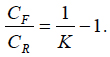

(17)

This formula indicates that if the availability index is high, the ratio of the cost of repairs to the cost aimed at improved reliability is low. When the availability index is low, this ratio is high. Again, this intuitively obvious result is quantified by the obtained simple relationship. The formula (16) can be used, particularly, to interpret the availability index from the cost-effectiveness point of view; the index reflects the ratio of the cost of improving reliability to the minimum total cost of the item associated with its reliability level.

The relationship between the availability index and cost-effectiveness of the product is quantified, assuming that the cost of improving reliability over its specified level increases, and the restoration (repair) cost decreases, when reliability level (assessed in our analysis by the mean-time-to-failure) increases. It has been shown that the total cost of improving and maintaining reliability can be minimized, and that such a minimized cost is inversely proportional to the availability index. The developed model can be of help when there is a need to minimize costs without compromising reliability.

References

1. E. Suhir, Applied Probability for Engineers and Scientists, McGraw-Hill, New York, 1997.
2. E. Suhir, R. Mahajan, A. Lucero and L. Bechou, “Probabilistic Design for Reliability (PDfR) and a Novel Approach to Qualification Testing (QT),” IEEE/AIAA Aerospace Conference, March 2012.

Ephraim Suhir, Ph.D., is Distinguished Member of Technical Staff (retired), Bell Laboratories’ Physical Sciences and Engineering Research Division, and is a professor with the University of California, Santa Cruz, University of Maryland, and ERS Co.; suhire@aol.com. Laurent Bechou, PH.D., is a professor at the University of Bordeaux IMS Laboratory, Reliability Group.

How one EMS company improved production time by shedding the straight line flow.

Two years ago, Orbit One decided to redesign its SMD line in Ronneby, Sweden, with the goal to decrease machines’ setup time or to increase uptime and shorten lead times.

The work started in 2010 when two “straight” production lines were reconfigured into a “U” shape, under the theory that this would minimize setup time and improve production flow.

To do so, we took two of our three lines and put them together. In other words, we took four placement machines and split assembly across the four modules, setting up the placement heads to assemble at the same time but just using half the number of feeders.

This way we shortened the lead time, and by using just one of the two feeder boards in the machines, we could perform a setup while simultaneously running the machines for the present job. That positively impacted uptime.

To optimize after this redesign, we adjusted the modules to balance the assembly time, which is of course important because the module with the longest assembly time determines the output from the machine. In theory it is simple, but it does require some effort from operators and programmers to make these movements between the modules. Depending on the design and number of components, some boards are harder to optimize. Also, other potential bottlenecks in the line, such as the screen printer or oven, must be considered.

Overall, the reconfigured line has been very successful. We produce with increased efficiency compared with the previous line configuration, and it’s easier to change production plans closer to the start date compared with the previous layout. Moreover, overall setup time has been decreased approximately 50%.

Per Jennel is sales and marketing manager at Orbit One (orbitone.se); per.jennel@orbitone.se.